This blog introduces the concept of System Identification and does so as applied to a BLDC Motor.
One purpose of identification is to identify the transfer function dynamics of the system. The systems can have various amounts of information known; ranging from full information (White Box), partial information (Grey Box) or no information (Black Box).
The application I am starting with is wanting to know the transfer function of a closed loop speed control of a BLDC motor.
Background
To identify a SISO transfer function we could just run a Bode plot. This is comprised of driving the input, u(k), with a swept sine and computing the output gain and phase by analyzing the output y(k) relative to the input u(k). An alternative to using a swept sine is to use a Pseudo Random Binary Signal (PRBS) implemented with a Linear Feedback Shift Register (LFSR). The LFSR represents an N bit polynomial. Once initialized the register is shifted every sample period, Ts. The new register contents are based on the present contents exclusive Ored on certain bits to implement a specific polynomial, A(N). If the polynomial has N bits, then there is 2^N-1 unique sequences before the shift register repeats. For example, for PRBS7 this denotes is a 7-bit shift register and it repeats after 127 clocks (2^7-1). Consider PRBS16 with Ts=1ms. There are 65535 unique values spanning a period of 65.5 seconds before the pattern repeats.
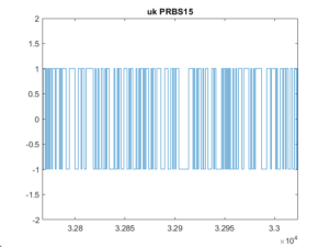
The figure below shows a slice of the PRBS15. It is scaled to amplitude values +/-1.
Denote the impulse response of a discrete system as h(k) with input u(k) and output y(k) then the output can be defined by the convolution equation:
$$y(k) = \sum_{-\infty}^{\infty} h(k-\tau) \cdot u(\tau)$$
The cross correlation of the input and output yields
$$Ruy(k) = \sum_{-\infty}^{\infty} y(k-\tau) \cdot u(\tau)$$ or
$$Ruy(\tau) = h(\tau) * Rxx(\tau)$$
In the frequency domain this can be written as,
$$Suy(f) = H(f) \cdot Sxx(f)$$
If u(k) is persistently exciting then Rxx is an impulse and Sxx is broadband which leads to Suy(f) being the spectrum of H(f).
Basic Steps
The basic steps are the following:
1. Drive the system input with a PRBS signal, u(k), with zero mean and amplitude +/-M.
2. Collect the response y(k) of the system.
3. Remove the mean from y(k) and calculate r(k), the cross-correlation of u(k) and y(k), using MATLAB xcorr().
4. Perform spectrum analysis on r(k) using MATLAB spa
As an example consider the transfer function below with Ts=5E-3.
$$G(z) = 0.20(z-0.95)/(z-0.5)(z-0.91)(z-0.8)$$
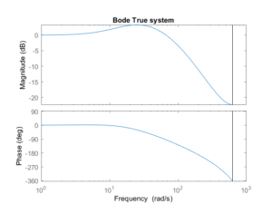
A Bode plot of this is shown in figure 1. This is our test system we wish to identify.
The following MATLAB code generates a PRBS16 signal for u(k) which is 2^16-1 sample periods and amplitude levels +/-1. The output of the system, y(k) is then computed using the dlsim command. The data set {u(k), y(k)} is spectrally analyzed using the spa(z) command from the MATLAB System ID Toolbox. This was run first with the case where there is no noise added to y(k) and then with noise added.
| %% System ID Example | |
| % Aug 5, 2021 | |
| % Uses MATLAB System ID Toolbox | |
| %% Generate u(k) | |
| Band= [0 1]; | |
| Range= [-1 1]; % amplitude limits | |
| Ts=5E-3; | |
| N=2^16-1; % # points | |
| % | |
| uk = idinput(N,'prbs',Band,Range); | |
| uk = uk - mean(uk); | |
| figure(1); stairs(uk);title('uk PRBS15'); axis([ N/2 N/2+256 -2 2]) | |
| %% Define 'True' system TF | |
| gn= 0.20; | |
| num= gn*[1 -0.95]; | |
| den= conv([1 -0.9], [1 -0.5]); | |
| den= conv([1 -0.80],den); | |
| figure(2); dbode(num,den,Ts); title('Bode True system') | |
| A2= axis; | |
| %% Compute y(k) w/ noise (if enabled) | |
| y= dlsim(num, den,uk); | |
| e = 2.0*(rand([N,1])-0.5); % add noise | |
| yk= y + 1*e; | |
| figure(3); stairs(yk); title('yk'); axis([ N/2 N/2+256 -2 2]) | |
| %% Show xcorr x & y | |
| r= xcorr(uk,yk); | |
| figure(4); stairs(r); title('xccor xk, yk') | |
| %% remove mean from u(k)and y(k)then analyze spectrum | |
| u2 = uk - mean(uk); | |
| y2 = yk - mean(yk); | |
| z = iddata(y2,u2,Ts); | |
| wz= logspace(-1,log(1*pi*200)/log(10),128); | |
| figure(5); bode(spa(z,500,wz),wz); title('Bode from sys ID spa') | |
| axis(A2) | |
| %% Plot pole-zero plot of True system | |
| figure(6); pzmap(tf(num,den)) |
The next figure shows the PRBS15 u(k) signal with noise added. In this case the noise was uniformly distributed over +/-1.
Figure 2 - Noisy u(k)
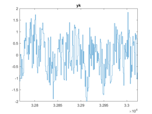
The next figure is the captured noisy y(k) signal.
Figure 3 - Noisy y(k)
From the captured {u(k), y(k)} signal pair we then use the MATLAB spa() function to analyze the spectrum. The Bode is shown here:
Figure 4 - System ID Noisy Bode
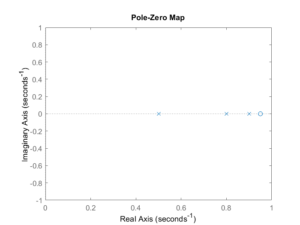
This last figure shows the pole-zero map of the True Bode.
Figure 5 - True System pole-zero map
The System ID with a noisy system shows a remarkably accurate result. The low frequency gain is unity and the phase lead results in an amplitude gain up to the point the other poles come into play. At high frequency (1/Ts) the phase shift shows 360 degrees due to the three poles and one zero.
This investigation was done in a MATLAB simulation but the follow-on blog will perform the real system ID in a setup using a STM32 MCU and BLDC motor looking at the closed velocity loop.


